Click Links Below to Navigate to Example Cases:
- Steady Example – Tactical Fighter
- Steady Example – Power BCs
- Time-accurate Example – Sod Shock Tube
- Steady Example – Forced Transition
The first example case demonstrates a typical, steady-state simulation using USM3D-ME.
For this case, an unstructured, mixed-element, half-span grid was generated. The grid includes 1,511,114 cells and is shown below.

The simulation was performed for Mach 0.75, 5,839.6 Reynolds number per grid unit, and 3 degrees angle of attack. Additionally, the Roe scheme was utilized for the inviscid flux calculations along with the one-equation Spalart-Allmaras turbulence model with negative provisions and the Quadratic Constitutive Relation (QCR-2000). Finally, HANIM was used for the nonlinear iterations, which features CFL adaptation to automatically adjust the CFL number for both the mean flow and turbulence equations as needed throughout the simulation. The convergence history, including CFL number and flow residuals versus iterations, is provided below.


Additionally, the iterative histories are provided below for the lift, drag, and pitching moment coefficients.


Finally, the figure below provides a contour plot of the surface pressure coefficient for the tactical fighter.

Example 2: Power Boundary Conditions
Example 2 illustrates the application of power boundary conditions for engine simulations.
The selected case is referred to as the 2D Coflowing Jet, which is described in detail at https://turbmodels.larc.nasa.gov/shear.html. This case consists of two jets separated by a two thin plates. The inner jet has a Mach number near 0.5 and the outer jet has Mach number near 0.25. The provided grid has unit span and extends from x = -10 to x = 200. Note that the separating plate extends from x = -10 to x = 0. Additionally, the provided grid is half-span (z-symmetry plane at z = 0) and consists of 327,680 hexahedral elements. Images of the y = 0 symmetry plane are provided below.


The simulation was performed with reference conditions defined as Mach 0.5, 50,000 Reynolds number per grid unit, and 0 degrees angle of attack. The 10102 boundary condition was applied to both the inner and outer jets. For the inner jet, the 10102 is applied to enforce a Pt/Pref = 1.1862 and Tt/Tref = 1.05. Similarly, the 10102 BC is applied to the outer jet to enforce Pt/Pref = 1.046 and Tt/Tref = 1.0. The Roe scheme was utilized for the inviscid flux calculations along with the one-equation Spalart-Allmaras turbulence model with negative provisions. Finally, HANIM was used for the nonlinear iterations, which features CFL adaptation to automatically adjust the CFL number for both the mean flow and turbulence equations as needed throughout the simulation. The convergence history is provided below.


The resulting centerline velocity at the z = 0 is shown below.

Example 3: Time-Accurate Simulation
The example case chosen to illustrate the time-accurate functionality is the Sod Shock Tube problem, which is an internal flow problem in a constant-area cylinder.
The problem is set up to enforce density and pressure gradients in the tube by applying rho, p, and u to 1.0, 1.0, 0.0 to the left boundary and 0.125, 0.1, and 0.0 to the right boundary. For this problem, an inviscid grid was generated consisting of 21,903 tetrahedral elements. An illustration of the grid is shown below for reference.

The example case is set up to run in time-accurate mode for a simulation time of 0.2 seconds to enable comparisons to the known analytical solution. The selected time step size was 0.002 seconds and the simulation is performed for 100 time steps. For each time step, 50 subiterations were imposed with the resstep input set to -12. The resstep input allows the code to break out of the subiterative loop early if the residuals drop by the user-specified value of resstep. This can help reduce computational cost and provide consistent convergence at each time step. The simulation was performed inviscid and applies the Roe scheme for the inviscid fluxes along with the Barth-Jesperson flux limiter. Finally, HANIM was used for the nonlinear iterations, which features CFL adaptation to automatically adjust the CFL number as needed throughout the simulation. The subiterative history of the mean flow residual is shown below.

The resulting Mach contour plot at t = 0.2 seconds is shown below.

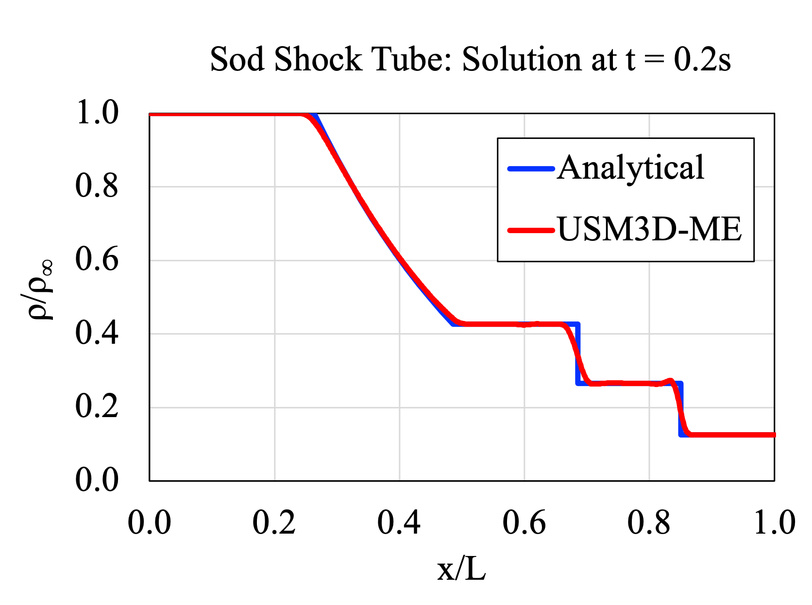
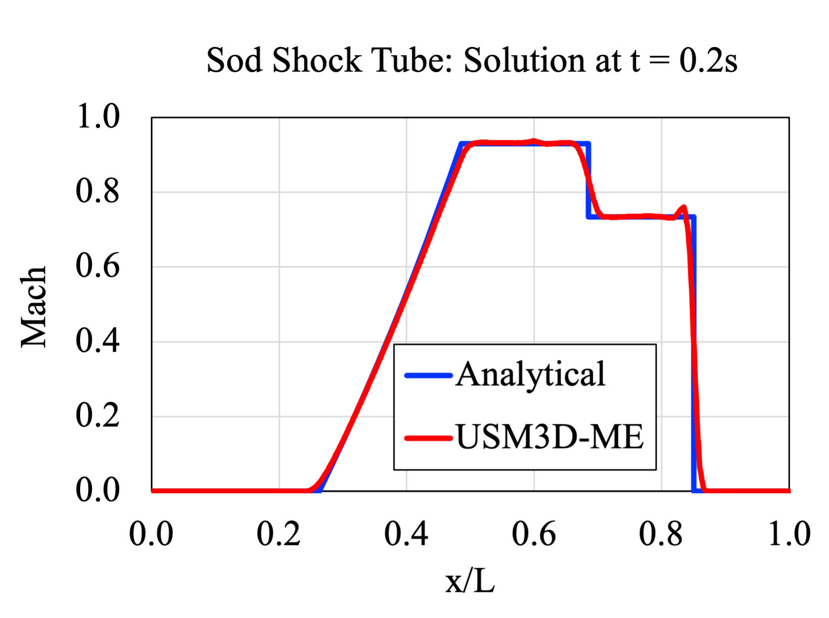
Finally, the centerline density and Mach number are plotted and compared to the analytical solution at t = 0.2 seconds.
Example 4: Steady Example – Forced Transition
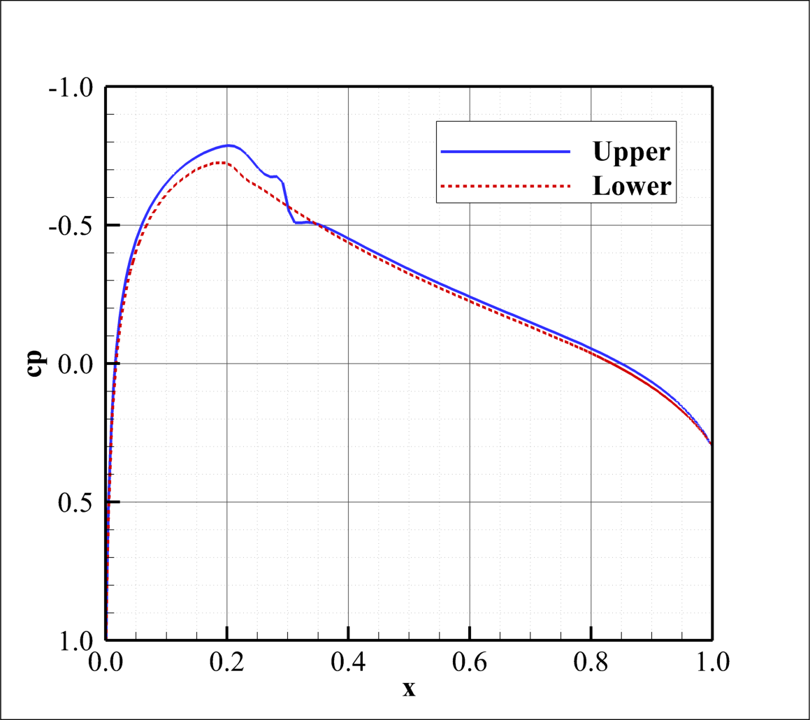
This example case illustrates the process for performing simulations with forced transition to turbulent flow. The case considers performing a steady simulation for a NACA 0012 airfoil with forced transition at x/c = 0.3.
For this example, a quasi-3D grid was generated with unit chord and span of 0.02. The grid was generated in two steps. First, a 2D, all tetrahedral grid was generated. Then, the 2D grid was extruded in the y-direction to produce a 3D representation of the problem. The resulting grid consists of 117,403 prismatic elements. An illustration of the grid on the y = 0 symmetry plane is shown below.


The simulation was performed with reference conditions defined as Mach 0.75, Reynolds number per grid unit = 10 million, and 0 degrees angle of attack. Note that an additional input file (proj_name.tran) is required for forced transition simulations. See the provided README file for instructions on how to generate this file.
The Roe scheme was utilized for the inviscid flux calculations along with the one-equation Spalart-Allmaras turbulence model with negative provisions, Rotation Correction, and Quadratic Constitutive Relation (QCR-2000). Finally, HANIM was used for the nonlinear iterations, which features CFL adaptation to automatically adjust the CFL number for both the mean flow and turbulence equations as needed throughout the simulation. The convergence history, including CFL number and flow residuals versus iterations, is provided below.


Additionally, the iterative histories are provided below for the lift, drag, and pitching moment coefficients.


Finally, plots of both skin friction magnitude and pressure coefficient are provided below.